Reference-guide transcriptome analysis
STAR比对的特点:速度快;准确度高
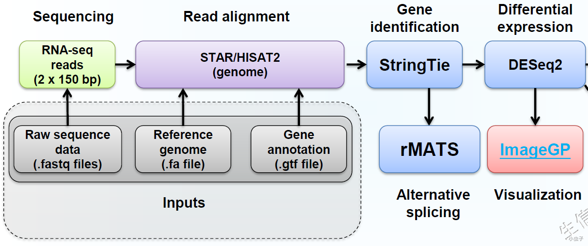
转录组有参分析之STAR比对及可变剪切
STAR比对的特点:
- 速度快
- 准确度高
- 3’reads soft clip
- genomeLoad LoadAndKeep 多个比对共享内存中的基因组索引 减小内存的使用量
- 直接获得基因的 reads count 和 导入基因组浏览器的 biwWig 文件
STAR转录组比对和定量

基因注释文件准备:gtf转bed12
gtfToGenePred -ignoreGroupsWithoutExons GRCh38.gtf GRCh38.gtf.50505050.pred
genePredToBed GRCh38.gtf.50505050.pred GRCh38.gtf.bed12
`选择长度适中的转录本用于后续评估`
awk '$3-$2>1000 && $3-$2<2000' GRCh38.gtf.bed12 >GRCh38.model.gtf.bed12
head GRCh38.gtf.bed12
STAR构建基因组索引
# 需要GTF文件中有exon\gene_id\transcript_id
cd ~/transcriptome/data/genome
mkdir -p star_GRCh38
# --runThreadN 2: 指定使用2个线程
# --sjdbOverhang 100: 默认
STAR --runMode genomeGenerate --runThreadN 2 --genomeDir star_GRCh38 \
     --genomeFastaFiles GRCh38.fa --sjdbGTFfile GRCh38.gtf
 ls -sh star_GRCh38

# 总用量 2.1G
# 4.0K chrLength.txt      368K exonInfo.tab          1.5G SAindex
# 4.0K chrNameLength.txt   24K geneInfo.tab          204K sjdbInfo.txt
# 4.0K chrName.txt         64M Genome                204K sjdbList.fromGTF.out.tab
# 4.0K chrStart.txt       4.0K genomeParameters.txt  204K sjdbList.out.tab
# 732K exonGeTrInfo.tab   516M SA                    224K transcriptInfo.tab
# STAR解析后的基因数
wc -l star_GRCh38/geneInfo.tab

# 原始GTF的基因数
grep -cP '\tgene\t' GRCh38.gtf
Reads比对
# mkdir新建目录
cd ~/transcriptome/data
mkdir -p trt_N061011

# 动物一般写 1000000,植物一般写5000
max_intron_size=1000000

# --genomeLoad LoadAndKeep : 共享内存
# 使用STAR比对的结果拼装时,一定要加比对参数`--outSAMattrIHstart 0 --outSAMstrandField intronMotif`
# 不然出来的都是单外显子转录本。

star_p=" --outFilterType BySJout --outSAMattributes NH HI AS NM MD \
       --outFilterMultimapNmax 20 --alignSJoverhangMin 8 --alignSJDBoverhangMin 1 \
       --alignIntronMin 20 --alignIntronMax ${max_intron_size} \
                --alignMatesGapMax ${max_intron_size} \
                --outFilterMatchNminOverLread 0.66 --outFilterScoreMinOverLread 0.66 \
                --winAnchorMultimapNmax 70 --seedSearchStartLmax 45 \
                --outSAMattrIHstart 0 --outSAMstrandField intronMotif \
                --genomeLoad LoadAndKeep --outReadsUnmapped Fastx \
                --outSAMtype BAM Unsorted --quantMode TranscriptomeSAM GeneCounts"

# STAR比对单个样品
nohup STAR --runMode alignReads --runThreadN 4 \
        --readFilesIn trt_N061011_1.fq.gz trt_N061011_2.fq.gz \
        --readFilesCommand zcat --genomeDir genome/star_GRCh38 \
        --outFileNamePrefix trt_N061011/trt_N061011. ${star_p} &

# --runThreadN 4: 使用4个线程
# --readFilesIn: 输入文件,左端和右端
# --readFilesCommand zcat:gzip压缩,指定解压方式
# --genomeDir:基因组索引目录的位置
# -S: 指定输出文件

# trt_N061011.ReadsPerGene.out.tab: 每个基因的reads count,链非特异性RNASeq选第2列.
# column 1: gene ID
# column 2: counts for unstranded RNA-seq
# column 3: counts for the 1st read strand aligned with RNA (htseq-count option -s yes)
# column 4: counts for the 2nd read strand aligned with RNA (htseq-count option -s reverse)


#筛选reads,按坐标排序、索引BAM文件供下游使用, 也可导入IGV查看reads比对情况、是否有变异位点等

# samtools具体参数解释见 samtools -?
# -@ 4: 4个线程
cd ~/transcriptome/data
mkdir -p tmp
samtools sort -@ 4 -T tmp/trt_N061011 \
  -o trt_N061011/trt_N061011.Aligned.sortedByCoord.out.bam \
  trt_N061011/trt_N061011.Aligned.out.bam
samtools index trt_N061011/trt_N061011.Aligned.sortedByCoord.out.bam
# 为什么要按坐标排序?
# 为什么要建索引?
# 就可以导入IGV中查看reads的比对情况了


# BigWig峰图文件生成,导入IGV或UCSC genomebrowser获取表达丰度图。

# Wig里面有什么?
# 为什么要生成BigWig?
# 是否需要标准化?
## BAM转BigWig
STAR --runMode inputAlignmentsFromBAM \
        --inputBAMfile trt_N061011/trt_N061011.Aligned.sortedByCoord.out.bam \
        --outWigType bedGraph --outFileNamePrefix trt_N061011/trt_N061011. \
        --outWigNorm RPM --outWigStrand Unstranded
bedSort trt_N061011/trt_N061011.Signal.UniqueMultiple.str1.out.bg \
        trt_N061011/trt_N061011.Signal.UniqueMultiple.str1.out.bg
bedGraphToBigWig trt_N061011/trt_N061011.Signal.UniqueMultiple.str1.out.bg \
        genome/star_GRCh38/chrNameLength.txt \
        trt_N061011/trt_N061011.Signal.UniqueMultiple.str1.out.bw

比对质量评估–RSeQC
### Reads在基因上的分布评估

# 程序运行结束后,默认生成折线图
geneBody_coverage2.py -i \
  trt_N061011/trt_N061011.Signal.UniqueMultiple.str1.out.bw \
  -r genome/GRCh38.model.gtf.bed12 -o trt_N061011/trt_N061011.geneBody_coverage

### Reads比对到基因组标志性区域的分布
read_distribution.py -i trt_N061011/trt_N061011.Aligned.sortedByCoord.out.bam \
  -r genome/GRCh38.gtf.bed12 >trt_N061011/trt_N061011.read_distrib.xls

cat trt_N061011/trt_N061011.read_distrib.xls


### 测序饱和度评估
# -s: 采样频率,0-100之间的整数,类似于步长
# -q: 过滤低质量比对
RPKM_saturation.py -i \
  trt_N061011/trt_N061011.Aligned.sortedByCoord.out.bam \
  -r genome/GRCh38.gtf.bed12 -s 10 -q 0 -o trt_N061011/trt_N061011.RPKM_saturation

ls -ltr trt_N061011l
批量比对和定量
for i in `tail -n +2 sampleFile | cut -f 1`; do
  mkdir -p ${i}
  mkdir -p tmp
  STAR --runMode alignReads --runThreadN 4 \
        --readFilesIn ${i}_1.fq.gz ${i}_2.fq.gz \
        --readFilesCommand zcat --genomeDir genome/star_GRCh38 \
        --outFileNamePrefix ${i}/${i}. ${star_p}
    samtools sort -@ 10 -T ${i}.tmp \
                -o ${i}/${i}.Aligned.sortedByCoord.out.bam \
                ${i}/${i}.Aligned.out.bam
  samtools index ${i}/${i}.Aligned.sortedByCoord.out.bam
  STAR --runMode inputAlignmentsFromBAM \
        --inputBAMfile ${i}/${i}.Aligned.sortedByCoord.out.bam \
        --outWigType bedGraph --outFileNamePrefix ${i}/${i}. \
        --outWigNorm RPM --outWigStrand Unstranded
    bedSort ${i}/${i}.Signal.UniqueMultiple.str1.out.bg \
        ${i}/${i}.Signal.UniqueMultiple.str1.out.bg
    bedGraphToBigWig ${i}/${i}.Signal.UniqueMultiple.str1.out.bg \
        genome/star_GRCh38/chrNameLength.txt \
        ${i}/${i}.Signal.UniqueMultiple.str1.out.bw
done &


## 批量评估

cd ~/transcriptome/data
for i in `tail -n +2 sampleFile | cut -f 1`; do
  geneBody_coverage2.py -i \
    ${i}/${i}.Signal.UniqueMultiple.str1.out.bw \
    -r genome/GRCh38.model.gtf.bed12 -o ${i}/${i}.geneBody_coverage
  read_distribution.py -i ${i}/${i}.Aligned.sortedByCoord.out.bam \
    -r genome/GRCh38.gtf.bed12 >${i}/${i}.read_distrib.xls
  RPKM_saturation.py -i \
    ${i}/${i}.Aligned.sortedByCoord.out.bam \
    -r genome/GRCh38.gtf.bed12 -s 10 -q 0 -o ${i}/${i}.RPKM_saturation
done &

## multiqc整理软件运行结果

multiqc -f -d . -o multiqc

## 合并表达文件

# 基因reads count增加样品信息,方便后续合并
# sed '5 i\Gene\ttrt_N061011\ttrt_N061011\ttrt_N061011' trt_N061011/trt_N061011.ReadsPerGene.out.tab trt_N061011/trt_N061011.ReadsPerGene.out.tab.ehbio

cd ~/transcriptome/data
for i in `tail -n +2 sampleFile | cut -f 1`; do
  sed "5 i\Gene\t${i}\t${i}\t${i}" ${i}/${i}.ReadsPerGene.out.tab >${i}/${i}.ReadsPerGene.out.tab.ehbio
done


# Linux 命令合并
cd ~/transcriptome/data
paste `find . -name *.ReadsPerGene.out.tab.ehbio` | tail -n +5 | \
  awk 'BEGIN{OFS=FS="\t" }{line=$1; \
    for(i=2;i<=NF;i++) if(i%2==0 && i%4!=0) line=line"\t"$i; print line;}' \
  >ehbio_trans.Count_matrix.xls
head ehbio_trans.Count_matrix.xls
鉴定新基因或转录本
## 转录本拼装

使用STAR比对的结果拼装时,一定要加比对参数`--outSAMattrIHstart 0 --outSAMstrandField intronMotif`,不然出来的都是单外显子转录本。

#单样本拼装


# # -G: 指定reference GTF
# -p 1: 使用一个线程,多核处理器可调大
# -f 0.01 : 允许的最小isoform比例,默认0.01

cd ~/transcriptome/data
stringtie trt_N061011/trt_N061011.Aligned.sortedByCoord.out.bam \
  -G genome/GRCh38.gtf -l trt_N061011 -o trt_N061011/trt_N061011.stringtie_first.gtf \
  -f 0.01 -p 2

# 多样本循环拼装

cat sampleFile

cd ~/transcriptome/data
for i in `tail -n +2 sampleFile | cut -f 1`; do
  stringtie ${i}/${i}.Aligned.sortedByCoord.out.bam -G genome/GRCh38.gtf -l ${i} -o ${i}/${i}.stringtie_first.gtf -f 0.01 -p 1
done &


# 转录本合并
cd ~/transcriptome/data
# 获取所有拼装好的gtf文件
find . -name *.stringtie_first.gtf >mergeList.txt

# -G: 指定reference GTF
# -l: 输出结果中转录本的名字前缀
# -o: 输出文件
# mergeList.txt:单个样品GTF列表,每个一行

stringtie --merge -G genome/GRCh38.gtf -l ehbio_trans -o ehbio_trans.gtf mergeList.txt


#新拼装转录本与原基因组注释转录本比较 (可用来筛选新转录本)

# -R: 只考虑与拼装的转录本有重叠的注释转录本
# -r: reference gtf
# -o: 输出前缀

cd ~/transcriptome/data
gffcompare -R -r genome/GRCh38.gtf -o assembeCompare2Ref ehbio_trans.gtf
# 会输出一个assembeCompare2Ref.annotated.gtf,用于后续的定量

输出文件:
sampleA2GRCh38.stats (总的数据统计)
sampleA2GRCh38.combined/annotated.gtf (query gtf信息)
sampleA2GRCh38.sampleA.stringtie_first.gtf.refmap  (原注释与组装转录本
的匹配信息)
sampleA2GRCh38.sampleA.stringtie_first.gtf.tmap (最匹配的原注释与组装
转录本的匹配信息)
sampleA2GRCh38.loci (转录本在基因组上的坐标信息)
sampleA2GRCh38.tracking (Tracking transfrags through multiple samples)

统计不同种类转录本的数目

cut -f 3 assembeCompare2Ref.ehbio_trans.gtf.tmap | tail -n +2 | sort | uniq -c
转录本定量
## 基于HTSEQ

for i in `tail -n +2 sampleFile | cut -f 1`; do
  htseq-count -f bam -r pos -a 10 -t exon -s no -i gene_id -m union ${i}/${i}.Aligned.sortedByCoord.out.bam assembeCompare2Ref.annotated.gtf >${i}/${i}.readsCount
  grep -v '^__' ${i}/${i}.readsCount | sed "1 iGene\t${i}"  >${i}/${i}.readsCount2
done &

## 基于Salmon
根据基因组及注释文件提取转录本
## 自己完成
差异剪接分析(alternative_splicing)
# -b1, -b2参数的值是一个文件,文件内是一个样品多个重复的bam文件
# 所有bam文件写在一行,用逗号隔开
# 下面例子中考虑到每行能展示的宽度有限,所以文件内容做了换行处理,实际是一行
cd ~/transcriptome/data
cat <<END >trt.bam.txt
./trt_N052611/trt_N052611.Aligned.sortedByCoord.out.bam,./trt_N061011/trt_N061011.Aligned.sortedByCoord.out.bam,./trt_N080611/trt_N080611.Aligned.sortedByCoord.out.bam,./trt_N61311/trt_N61311.Aligned.sortedByCoord.out.bam
END

cat <<END >untrt.bam.txt
./untrt_N052611/untrt_N052611.Aligned.sortedByCoord.out.bam,./untrt_N061011/untrt_N061011.Aligned.sortedByCoord.out.bam,./untrt_N080611/untrt_N080611.Aligned.sortedByCoord.out.bam,./untrt_N61311/untrt_N61311.Aligned.sortedByCoord.out.bam
END

# --gtf: 指定基因注释文件,可以是自己下载的注释,也可以是stringtie拼装完merge后的注释
# --od: 输出目录 (output dir)
# -t: paired-end or single-end
# --libtype: 链特异性类型
# -nthread: 多线程计算; --tstat: 统计模型多线程计算
# --cstat: 差异剪接阈值,默认0.0001, 表示有0.01%的差异,取值在0-1之间

rmats.py --b1 trt.bam.txt --b2 untrt.bam.txt --gtf genome/GRCh38.gtf --od trt_untrt -t paired --libType fr-unstranded --readLength 63 --nthread 2 --tstat 2 --cstat 0.0001


#筛选差异显著的剪接位点

awk 'FNR==1 || $20<0.2' trt_untrt/SE.MATS.JC.txt >trt_untrt/SE.MATS.JC.sig.txt

head trt_untrt/SE.MATS.JC.sig.txt

#  sashimiplot

# --b1, --b2 同rMATS,只是直接跟文件内容而不是文件名
# -t: 想要绘制的类型
# -e: rMATS的输出,一般选择差异显著的绘制
# --exon_s,  --intron_s: 缩放外显子或内含子,默认无缩放;一般用于内含子太大时,把内含子
# 相对缩小一点,图会更好看一些
# --l1, --l2,对应于--b1, --b2的样品的组名
# -o 指定输出目录

rmats2sashimiplot --b1 ./trt_N052611/trt_N052611.Aligned.sortedByCoord.out.bam,./trt_N061011/trt_N061011.Aligned.sortedByCoord.out.bam,./trt_N080611/trt_N080611.Aligned.sortedByCoord.out.bam,./trt_N61311/trt_N61311.Aligned.sortedByCoord.out.bam --b2 ./untrt_N052611/untrt_N052611.Aligned.sortedByCoord.out.bam,./untrt_N061011/untrt_N061011.Aligned.sortedByCoord.out.bam,./untrt_N080611/untrt_N080611.Aligned.sortedByCoord.out.bam,./untrt_N61311/untrt_N61311.Aligned.sortedByCoord.out.bam -t SE -e trt_untrt/SE.MATS.JC.sig.txt --exon_s 1 --intron_s 5 --l1 trt --l2 untrt -o trt_untrt/SE.MATS.JS.sig.sashimiplot


STAR定量结果差异分析
## 文件准备

文件来源于流程`pipelineStar.sh`中合并后的基因表达`reads count`,以其为准。


## 初始化

使用时只需要修改 `ehbio_trans.Count_matrix.xls`和`sampleFile` 即可。分组信息列必须是`conditionds`,如果不是,下面代码中的`conditions`也需相应的修改。


# 所有输出结果的前缀,根据需要修改
ehbio_output_prefix = "ehbio_star"
ehbio_reads_count = "ehbio_trans.Count_matrix.xls"
# 分组信息列必须是`conditionds`,如果不是,下面代码中的`conditions`也许相应的修改
ysx_sampleFile_init = "sampleFile"


reads_count <- read.table(ehbio_reads_count, header=T,  row.names=1, sep="\t", com='', quote='', check.names=F)


sample <- read.table(ysx_sampleFile_init, header=T, row.names=1, com='',
  quote='', check.names=F, sep="\t")
sample <- sample[match(colnames(reads_count), rownames(sample)),, drop=F]

# 注意这个函数的不同
dds <- DESeqDataSetFromMatrix(countData=reads_count, colData=sample, design= ~conditions)
print(paste("Read in", nrow(dds),"genes"))
keep <- rowSums(counts(dds))>nrow(sample)/2
dds <- dds[keep,]
print(paste(nrow(dds),"genes remained after filtering of genes with all counts less than", nrow(sample)/2, "in all samples"))
License
Copyright 2021 Guo-Cheng Li. Released under the MIT license.
Guo-Cheng Li
PhD of cell biology
Hi! I am a PhD at Institute of Zoology, The Chinese Academy of Sciences, Beijing, China. I am using genomics and transcriptomics to study insect chemoreception.